In this section, we will explore the following questions.
What is a discrete dynamical system? How do they relate to sequences?
How can we use discrete dynamical systems to describe real-world phenomena like predator-prey interactions, or the spread of a disease in a population?
In Section 4.1, we introduced the notion of a sequence. In this section, we will focus on situations in which our sequences represent a quantity changing over discrete, consistent periods of time. We will also consider systems of sequences: two or more interrelated sequences which describe the behavior of multiple changing quantities all at once. Before we dive into such systems, we consider another type of growth.
Subsection4.2.1Exponential Growth
Populations of people and animals do not grow linearly. Instead, they usually grow by a percentage of the whatever the current population is. So, if that annual percentage is, say, 10%, and the current population of a group of fish in a pond is 1000, this model predicts a population of \(1000 + 10\%\cdot 1000 = 1000 + 100 = 1100\) fish for next year.
In symbols, if \(P_t\) represents the number of fish \(t\) years from now, then \(P_0 = 1000\text{,}\)\(P_1 = P_0 + 0.1\cdot P_0 = (1+0.1)P_0 = 1.1 P_0\text{.}\) The number 0.1 is called the growth rate, \(r\text{,}\) and the number 1.1 is the growth multiplier.
In what follows, I will occasionally provide Sage cells in which you can do basic computations (and in which I may help get you started). To see how this works, click "Evaluate" in the Sage cell below to see what happens.
Exploration4.2.1.
Consider a population of 1000 fish growing at 10% per year.
Give a formula for \(P_2\) in terms of \(P_1\text{,}\) and then a formula for \(P_3\) in terms of \(P_2\text{.}\)
Using your answer to the previous part as a guide, give a formula for \(P_t\) in terms of \(P_{t-1}\text{.}\)
Again, using your answer to Question 1 and the work in the paragraph preceding this activity, give a formula for \(P_2\) in terms of \(P_0\text{.}\) Use this formula to find \(P_3\) in terms of \(P_0\text{.}\) Why might these formulas be more useful than the ones you found in Question 1?
State your best guess for a formula for \(P_t\) in terms of \(P_0\text{.}\) Use your formula to estimate the number of fish in the pond after 10, 20, and 50 years. What is this model missing?
Press “Evaluate” below to confirm your response to Question 4. What happens if you increase or decrease the growth rate, \(r\text{?}\) Try it, and reevaluate.
The type of growth explored in Exploration 4.2.1 called exponential, as the growth comes from taking the growth multiplier to larger and larger powers (exponents). We saw the danger of extrapolation with linear models in Activity 4.1.4, and we note a similar danger in extrapolating with exponential models. If nothing else, it’s likely that the pond cannot hold 100,000 fish. Thankfully, we can modify our exponential growth model by introducing an upper limit for what the habitat can hold.
Exploration4.2.2.
Suppose our pond can hold 5000 fish. This is known as the carrying capacity, and we’ll denote it with the letter \(K\text{.}\) We’ll now let \(r = 0.1\) be our maximum growth rate, but we’ll let it slowly reduce as the population grows.
As \(P_t\) increases and gets closer and closer to \(K\) over time, what happens to the ratio \(P_t/K\text{?}\) What number does it get close to?
Thus, what happens to the expression \(1-\frac{P_t}{K}\) as \(P_t\) increases and gets closer and closer to \(K\text{?}\)
Ecologically speaking, what does it mean for \(P_t\) to get closer and closer to \(K\text{?}\)
As the phenomena described in Question 3 occurs, what do we expect the graph of \(P_t\) over time to look like?
Test your suspicion by evaluating the Sage code below.
Subsection4.2.2A discrete predator-prey model
We now consider systems of discrete sequences, called discrete dynamical systems.
Definition4.2.3.
A dynamical system refers to any fixed mathematical rule which describes how a system changes over time. A discrete dynamical system changes at fixed intervals in time (e.g., each hour), and does not change between the fixed points in time (e.g., a system that changes each hour will view the changing quantity as static between the hours of 1:00pm and 2:00pm).
There are two main types of dynamical systems: discrete and continuous. The study of continuous dynamical systems is the domain of calculus and its related disciplines (e.g., differential equations). Continuous dynamical systems treat time as infinitely divisible; discrete dynamical systems do not. Typically, a dynamical system involves multiple related quantities that change over time.
We begin with a classic predator-prey model adapted from the Feedback Systems Wiki 1
at Caltech. For historical reasons, we let \(L_t\) be the size of a population of Canadian lynxes in year \(t\) and \(H_t\) be the size of a population of snowshoe hares, the lynx’s primary prey.
Definition4.2.4.
Let \(H_0\) be the initial population of hares, and \(L_0\) the initial population of lynxes. For \(t\ge 1\text{,}\) the discrete Lotka-Volterra model for the lynx/hare population is given by:
\begin{align*}
H_{t+1} \amp = H_t + b(u) H_t - a L_t H_t\\
L_{t+1} \amp = L_t + c L_t H_t - d L_t,
\end{align*}
where \(b\) is the hare birth rate per unit time as a function of the food supply \(u\text{,}\)\(d\) is the lynx mortality rate, and \(a\) and \(c\) are interaction coefficients.
Note the interrelationship between the two equations: the formula for calculating \(H_{t+1}\) requires knowing not only \(H_t\text{,}\) but also \(L_t\text{.}\) This makes sense! These populations interact, so the presence (or absence) of lynx should reasonably affect the hare population. Let’s further analyze this model.
Exploration4.2.5.
Consider the predator/prey model introduced in Definition 4.2.4.
What do the terms \(L_t\) and \(H_t\) represent?
Which term in the model represents an increase in the hare population? Which term represents a decrease in the hare population? Explain how you know.
Which term in the model represents an increase in the lynx population? Which term represents a decrease in the lynx population? Explain how you know.
may be helpful here; also consider what \(a\) is described to be.)
What simplifying assumptions does this model make about how the populations increase and decrease?
Activity4.2.6.
Let’s start by assuming that \(H_0 = 20\) and \(L_0 = 35\text{.}\) That is, we begin with 20 hares and 35 lynxes. Let’s further assume that \(a = c = 0.001167\text{,}\)\(b = 0.05\text{,}\) and \(d = 0.0583\) (parameters scaled by 12 months).
Compute \(H_1, H_2, L_1,\) and \(L_2\text{.}\) What seems to be happening to the two populations? Confirm using the Sage cell below, which will display the first ten months’ worth of predictions, or explore this spreadsheet 3
. Note that the hare population is given by the blue dots and the lynx population by the red.
The interaction coefficients translate to a decrease in the lynx population and an increase in the hare population. What do you expect to happen if we increase it from 0.014 to 0.05?
Test your suspicion using the Sage cell below, or this spreadsheet 4
Qualitatively describe the dynamics displayed in the Sage output in the previous question.
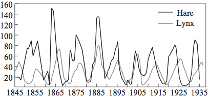
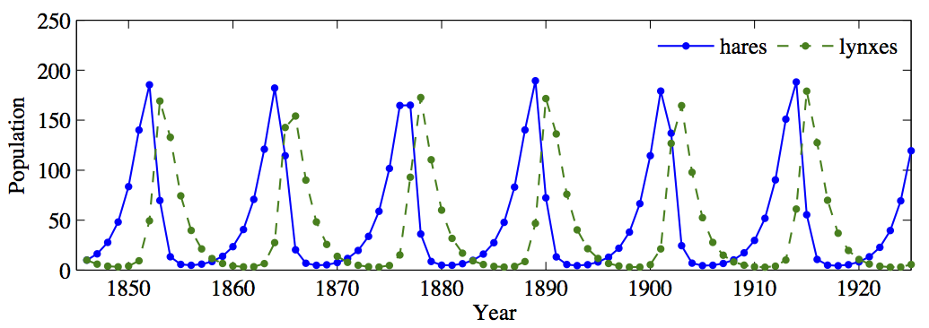
One might reasonably wonder how such a simple model does in making predictions about the long-term dynamics of these populations. The answer is: surprisingly well! In Figure 4.2.7, observe the actual collected data on hare and lynx populations over 90 years, from 1845 to 1935. In Figure 4.2.8, we see dynamics predicted by the model. Note the same cyclical patterns of an increase in the hare population followed by an increase in the lynx population, which in turn causes a decrease in the hare population, etc.
Figure4.2.7.Data on hare and lynx populations over time. (Source 5
To be clear, the purpose of the model is not to make absolutely certain predictions about the precise numbers of hares and lynxes present in the Canadian wilderness. Instead, we want to understand the broad dynamics of how the populations change relative to one another. Mathematical ecologists can then use these models to understand how small changes in the parameters (say, an increase in the rate of predation) affect the broader dynamics of the ecological system.
Subsection4.2.3The discrete SIR epidemiological model
We now arrive at the main goal of this chapter: the description of a basic mathematical model for the spread of an infectious disease. We’ll first present the model itself and examine its features and assumptions. As was the case with the predator-prey model, we’ll see that while it does make simplifying assumptions, it still allows us to analyze the broader dynamics of the disease transmission. We’ll then look at ways of reducing the rate of infection, including the so-called "flattening the curve" method.
We begin with the model. It is known as a compartmental model, as it divides the population into compartments and assumes that every individual in the same compartment has the same characteristics (at least as far as the transmission of the disease is concerned). We’ll look at the simplest such model, the discrete SIR model. Many more complex models are built on the SIR model.
Definition4.2.9.
Consider a population of \(N\) people through which a disease is spreading. For some discrete time \(t \ge 0\text{,}\) let \(S_t\) denote the number of individuals susceptible to the disease, \(I_t\) the number of individuals infected with the disease, and \(R_t\) the number of individuals who have recovered from the disease. We assume that that people move through the compartments as follows:
\begin{equation}
S \to I \to R.\tag{4.2.1}
\end{equation}
For \(t\ge 1\text{,}\) the model is given by the following equations.
\begin{align*}
N \amp = S_t + I_t + R_t\\
S_{t+1} \amp = S_t -b S_t I_t\\
I_{t+1} \amp = I_t + b S_t I_t - a I_t\\
R_{t+1} \amp = R_t + a I_t.
\end{align*}
The constant \(a\) is known as the recovery rate parameter, which roughly describes how fast someone moves from the infected compartment to the recovered compartment. The constant \(b\) is known as the infection rate, and roughly describes how fast someone moves from the susceptible compartment to the infected compartment.
Let’s explore the equations.
Exploration4.2.10.
What does (4.2.1) mean? What assumptions does this make? How does it simplify our analysis?
What does the first equation in the set of four mean? What assumptions does it make about the population?
The second equation describes how the susceptible population changes over time. It contains the term \(-b S_t I_t\text{.}\) Based on our work above with a predator-prey model and the definition of \(b\text{,}\) what epidemiological event is this term describing?
Explain why it makes sense that we add \(b S_t I_t\) in the equation defining \(I_{t+1}\text{.}\)
What does the term \(-a I_t\) mean in the equation for \(I_{t+1}\text{?}\) Why does it make sense to add\(a I_t\) in the equation for \(R_{t+1}\text{?}\)
Note that there are no terms being subtracted in the equation for \(R_{t+1}\text{.}\) What assumption does this tell us that the model is making?
Activity4.2.11.
Let’s see what happens when we plug in some numbers. Assume that \(N = 10,000\text{,}\)\(R_0 = 0\text{,}\) and \(I_0 = 50\text{.}\)
Why does it make sense that we have \(R_0 = 0\) (assuming we have a new disease entering a population).
What is \(S_0\text{?}\)
Let’s assume that \(a = 0.1\) and \(b = 0.0001\text{.}\) Compute \(S_1, I_1\text{,}\) and \(R_1\text{.}\)
Use your answer to the previous part to compute \(S_2, I_2\text{,}\) and \(R_2\text{.}\)
. Download the file and play around with the numbers at the top of the sheet to change some of the features; e.g., how does increasing/decreasing the number of initial infected individuals change the shape of the curves? What do you notice? What do you wonder? Give at least 2-3 observations or questions.
The COVID-19 pandemic introduced many people to a quantity called \(r_0\text{.}\) This is known as the basic reproduction number, and is the expected number of new infections directly generated by a single case. So, if Sam were to get COVID-19, \(r_0\) would be the expected number of people Sam would directly infect. We would then expect each of them to infect another \(r_0\) people, and so on.
Generally, if \(r_0 \gt 1\text{,}\) we expect the disease to spread. If \(r_0 \lt 1\text{,}\) we expect it to die out.
The next activity explores the ways in which varying \(r_0\) impacts new cases of the disease caused both directly and indirectly by a single person.
Activity4.2.13.
In this activity, we assume different values for \(r_0\text{.}\) However, we will make two assumptions that don’t change.
First, assume that all direct infections are done within a 5-day period. Second, assume that that those infected don’t infect others until the next five day period.
Let \(C_t\) be the number of cases I’ve caused after \(t\) five-day periods. Assume \(C_0 = 1\) (me).
Using that formula, what is the approximate \(r_0\) for the situation described in Activity 4.2.11?
Given that value of \(r_0\text{,}\) use the Sage cell below (replacing the ? with the value you found) to estimate how many cases Sam directly or indirectly causes over a 30-day period.
is intended to reduce \(r_0\text{.}\) Assume that strict social distancing is observed, and this reduces \(r_0\) to approximately 1.25 (one direct infection fewer). Now how many cases does Sam cause over the course of a 30-day period?
As the COVID-19 situation is ongoing, estimates for \(r_0\) vary significantly (and are variant-dependent). One study from February 2020 10
academic.oup.com/jtm/article/27/2/taaa021/5735319
found an average \(r_0\) of 3.28. If that is the true number, approximately how many cases will a typical infected person be responsible for over the course of a month? Use the Sage cell to determine your answer.
Other studies suggest that, in the absence of any social interventions, the original variant of COVID-19 has \(r_0 \approx 2.38\text{.}\) In that case, how many cases would an infected person be responsible for over the course of a month?
The Delta variant of COVID-19 has \(r_0 \approx 5.1\text{.}\) If I am infected with the Delta variant, approximately how many new cases will I cause within a month?
The Omicron variant of COVID-19 has an estimated \(r_0 \approx 10\) (note that this is being written in February 2022, just as the first major Omicron wave is subsiding; it should therefore be treated as preliminary). If Sam is infected with the Omicron variant, approximately how many new cases will he cause within a month?
For our last activity, we’ll explore how reducing \(r_0\) “flattens” the curve of infected people at time \(t\text{,}\)\(I_t\text{.}\) There are two main advantages of a flattened infected curve. First, this often corresponds to fewer infected people overall. Second, the lack of a spike in infected persons makes it easier for the healthcare system to effectively treat those who are infected (not to mention anyone with other medical concerns).
Exploration4.2.14.
One last time, consider the values for the variables we used in Activity 4.2.11; for reference, this was \(S_0 = 10000\text{,}\)\(I_0 = 50\text{,}\)\(R_0 = 0\text{,}\)\(a = 0.1\text{,}\) and \(b = 0.0001\text{.}\) We’ll again use the Google sheet 11
This value is pretty high (though it is approximately the \(r_0\) of diseases like measles and chicken pox!), but is convenient for our purposes. Nonetheless, we can still explore the ways in which changes in \(r_0\) affect the shape of the curves; our qualitative observations will still apply to real-world situations like the current coronavirus pandemic.
Recall that \(r_0 \approx \frac{bN}{a}\) and assume our population size \(N = 10000\) and recovery rate \(a = 0.1\) are constant. Compute the three values of \(r_0\) that result from infection rates of \(b = 0.00005, 0.0001\text{,}\) and \(0.0002\text{.}\) In turn, plug these values into the Google sheet 12
and comment on the shape of the infection curve: how tall is the spike of infected individuals, and at what time \(t\) is it at its highest point?
Similarly, assuming \(N = 10000\) and \(b = 0.0001\) are constant, compute the values of \(r_0\) that result from \(a = 0.05, 0.1\text{,}\) and \(0.2\text{.}\) In turn, plug these values into the Google sheet 13
and comment on the shape of the (green) infection curve: how tall is the spike of infected individuals, and at what time \(t\) is it at its highest point?
In this section, we first saw exponential growth, and discussed the strengths and weaknesses of using exponential growth to model a changing population. We also explored a basic predator-prey model, and noted that though the specific predictions made by the model may not be completely accurate, it does a good job of describing the broader dynamics and trends in the populations of the predator and prey.
We concluded by exploring a discrete version of the SIR epedimiological model, which is useful for describing the spread of a disease through a population. We used the model to test the effect of various interventions and observed how slowing the spread of the disease “flattens the curve” of infected individuals.
Exercises4.2.4Exercises
1.
The predator-prey model described in Definition 4.2.4 is known as a discrete Lotka-Volterra model. Do some research online to determine who Lotka and Volterra were, and what questions they were interested in. Write one or two paragraphs describing your findings.
2.
An advantage of the SIR model explored in this section is its simplicity: the population is split into only three compartments. However, through the use of more compartments it is possible to identify subtler dynamics at work; find such a model, such as an SEIR model, describe the choices it makes, and what is gained by the additional complexity.